
Navier-Stokes equation
$$\Large \dfrac{\partial\vec{\mathbf{v}}}{\partial t} + (\vec{\mathbf{v}}\cdot \nabla)\vec{\mathbf{v}} = – \dfrac{\nabla p}{\rho} + \nu \nabla^2 \vec{\mathbf{v}}$$
On the left side of the equation is the acceleration part.
$\dfrac{\partial\vec{\mathbf{v}}}{\partial t} \text{ – unsteady term}$
$(\vec{\mathbf{v}}\cdot \nabla)\vec{\mathbf{v}} \text{ – convective acceleration, nonlinear term}$
$\dfrac{\nabla p}{\rho} \text{ – pressure gradient, density is const.}$
$\nu \nabla^2 \vec{\mathbf{v}} \text{ – viscosity of newtonian fluid, 2nd order term}$
We solve 2nd order, nonlinear, partial derivative equation.
As solution we expect:
- The velocity field (vectors)
- The associated pressure (scalar)
Euler equation
For inviscid fluid $\Rightarrow \nu = 0$
Then we get the Euler equation:
$$\Large \dfrac{\partial\vec{\mathbf{v}}}{\partial t} + (\vec{\mathbf{v}}\cdot \nabla)\vec{\mathbf{v}} = – \dfrac{\nabla p}{\rho}$$
Model and discretize
1 – The mathematical model – Set of partial differential or integral-differential equation
Target application
- incompressible
- inviscid
- turbulent
- 2D or 3D
2 – The discretization method
Method for approximating the PDES by a system of algebraic equations
$\mathcal{L}[u(\underline{x})] = f(\underline{x}) \Rightarrow A\underline{x} = b$
Differential operator L is a function of x
- finite difference, FD
- finite volume, FV
- finite elements, FE
- spectral methods
- boundary element method, BEM
- particle methods
3 – Analyze the numerical scheme
All numerical schemes must satisfy certain conditions to be accepted:
- consistency
- stability
- convergence
Need for analyze the accuracy
4 – Solve
Obtain grid/point values of all flow variables
- time-dependent $\Rightarrow$ DDES – time integrators
- steady $\Rightarrow$ algebraic system of equations – linear solvers
Differential form of the Fluid Equations
1 – Conservation of Mass
For a system: $\dfrac{\mathrm d M_{sys}}{\mathrm d t}=0$
For a Control Volume: $\dfrac{\partial}{\partial t}\int_{cv}\rho\cdot\mathrm d V + \int_{cs}\rho\vec{\mathbf{v}}\cdot\hat{n}\cdot\mathrm d A = 0$
$\dfrac{\partial}{\partial t}\int_{cv}\rho\cdot\mathrm d V$ – Rate of change of mass in Control volume CV
$\int_{cs}\rho\vec{\mathbf{v}}\cdot\hat{n}\cdot\mathrm d A$ – Net rate of flow of mass across Control surfaces CS ($\hat{n}$ – normal, A – Area)
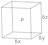
<u>Differential Form</u> – consider a small fluid element $\delta x \delta y \delta z$
-
$\dfrac{\partial}{\partial t}\int_{cv}\rho\cdot\mathrm d V = \dfrac{\partial\rho}{\partial t}\delta x \delta y \delta z$, $\rho$ is uniform in $\delta V$
-
Rate of mass flow: in the xyz-direction
$\left[ \rho u – \dfrac{\delta}{\delta x}(\rho u)\dfrac{\delta x}{2}\right]\delta y \delta z$ $\rightarrow$
$\rightarrow$ $\left[ \rho u + \dfrac{\delta}{\delta x}(\rho u)\dfrac{\delta x}{2}\right]\delta y \delta z$
Net rate of mass outflow in
x-direction: $\dfrac{\delta}{\delta x}(\rho u)\delta x \delta y \delta z$
y-direction: $\dfrac{\delta}{\delta y}(\rho v)\delta x \delta y \delta z$
z-direction: $\dfrac{\delta}{\delta z}(\rho w)\delta x \delta y \delta z$
$\Rightarrow \dfrac{\delta \rho}{\delta t} + \dfrac{\delta}{\delta x}(\rho u) + \dfrac{\delta}{\delta y}(\rho v)+\dfrac{\delta}{\delta z}(\rho w) = 0$
$\text{Vector notation}\rightarrow \dfrac{\delta \rho}{\delta t} + \nabla \cdot\rho\vec{\mathbf{v}} = 0$